Basic Usage¶

The main transform functions are stransform and istransform. They can be used simply, as in the following example.

Forward transform¶

import numpy as np
from scipy.signal import chirp
from particleman import stransform

sample_rate = 40.0  #[Hz]
total_sec = 30.0

# make a linear chirp
t = np.arange(0.,total_sec,1./sample_rate)
c = chirp(t, 0.2, 20.0, 10.0, method='linear', phi=0, vertex_zero=True)

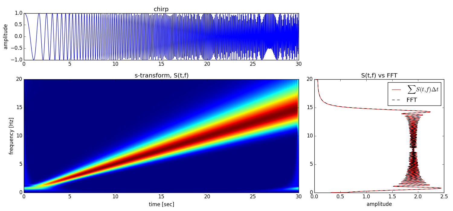
S, T, F = stransform(c, Fs=sample_rate, return_time_freq=True)

S is the time-frequency Stockwell tile, a 2D numpy.ndarray. T and F are the time and frequency domain grids for plotting S. As these can sometimes be large, you may use the return_time_freq=False keyword.

This example shows that a time-integration of the the Stockwell transform is equivalent to the traditional FFT.

chirp

Optionally, only certain rows of the S-transform can be returned (filtered), using the hp (high-pass) and lp (low-pass) keywords, which are in Hertz. This is useful if you know the frequency band of interest, or the return tile(s) are unmanageably large.

Inverse transform¶

The inverse transform has very similar syntax:

ctr = istransform(S, Fs=sample_rate)

np.allclose(c, ctr)

True